In the previous article, we learned together about what regression is. As I promised earlier, I will teach you a little bit about what I understand about how to use regression if the data we analyze is small. Regression analysis is known for its ease of use in various types of analysis, but can regression work if the dataset being analyzed is small? Is it different if the sample we analyze is 1000? Is it different if the sample analyzed is 20? How do we distinguish whether the regression we analyze is a coincidence or not?
Unlike other statistical methods that work well with large sample sizes, regression can still work well with small samples. One way to make regression analysis work well with small samples is to apply the t-distribution.
What is t-distribution?
The T-distribution, also known as the “student distribution,” is a method first introduced by William Sealy Gosset, who used the pen name “student” when publishing his scientific papers.
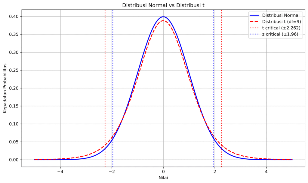
As can be seen from the image above, the t-distribution graph depicted by the dotted red line has a “fatter” tail compared to the normal distribution graph. The t-distribution is a way of depicting data that follows a normal distribution, which is bell-shaped. However, the ends of the tail are thicker. The t-distribution is used for small samples and when the data variation (the spread of data from the mean) is unknown.
Degree of freedom
The shape of the t-distribution graph is influenced by the Degree of Freedom (df). From now on, I will refer to the degree of freedom as df. Df is simply the number of samples observed (n) minus the observation limitations. For example, you are asked to find four numbers that add up to 100.
For example, you have already determined 3 numbers:
- Number- 1 = 20
- Number- 2 = 10
- Number- 3 = 40
Then we can no longer freely take the fourth number because there is a limit on the number of numbers added, which must be 100:
20 + 10 + 40 + x = 100 ⇒ x = 30
Since only 3 numbers can be chosen freely, the df is 3. Out of 4 choices, only 3 can be chosen freely and 1 must follow the set restrictions. Df = 4 – 1 = 3.
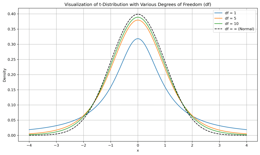
As you can see in the figure above, for a graph with df 1, the top of the graph tends to be shorter and both tails of the graph are thicker. Additionally, as df increases, the resulting graph has a higher top and thinner tails. As df increases, the graph will take on a shape that follows a normal distribution. Generally, df values above 30 will have a graph shape similar to a normal distribution.
Case study
After understanding the characteristics of the t distribution graph, which has a fatter shape than the normal distribution, we will now move on to the main discussion: how to use regression analysis when the observed data is small.
After comparing the graph shapes between the t-distribution and the normal distribution, if the graph shape is fatter than the normal distribution, we need to calculate the t-value and compare it with the t-distribution. If the t-value is greater than the t-distribution, our initial hypothesis is proven.
To understand this better, let’s look at the following case study. A teacher argued that the more hours of learning, the higher the grades his students would get. He then conducted an experiment, which consisted of 10 trials with learning durations ranging from one hour to eight hours. When the learning was complete, he administered a test.
| test number- | hour (x) | exam score (y) |
| 1 | 1 | 50 |
| 2 | 2 | 55 |
| 3 | 2 | 53 |
| 4 | 3 | 60 |
| 5 | 4 | 62 |
| 6 | 4 | 61 |
| 7 | 5 | 65 |
| 8 | 6 | 70 |
| 9 | 7 | 74 |
| 10 | 8 | 78 |
After conducting ten experiments, the results were obtained as shown in the table above. The linear regression equation was calculated. You can use applications such as Excel, Tableau, or Python. The equation obtained was:
Y = 48 + 3.5X
t-value calculation
This means that for every additional hour, the value obtained will increase by approximately 3.5. Due to the small number of samples, we need to test whether x is a coincidence or not.
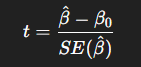
- β = 3.5. Estimated results, you can see the previous equation.
- β0 = 0 null hypothesis value (no effect)
- SE(β) = 0.8. standard error coefficient
T-distribution calculation
After performing the calculation, the t-value obtained is 4.375. The next step is to calculate the t-distribution. You can find this value using a t-distribution table or an online t-distribution calculator. Since n = 10, the degrees of freedom (df) = 10 – 2 = 8. Refer to the t-table for df = 8 and a significance level of 0.05 → the critical value is approximately ± 2.31.
|t| = 4.375 > 2.31
Thus, the duration of study hours has a significant effect on improving students’ grades. With t distribution, we can still use regression even though the sample used is quite small.
Also read: Regression, a Method for 1000 Problems