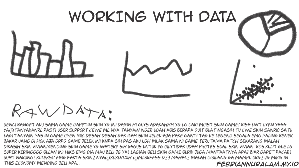
Working with data is like a combination of art and science. But people tend to focus only on the scientific aspect. Today, we’ll explore the artistic side.
Exploratory Data Analysis (EDA)
Once you’ve decided on the question you want to answer and you have the data you need, you’re probably eager to jump right in and build a machine learning model to get the answer to your question. But the first step you need to take is to explore the data you have.
One-dimensional data exploration
One-dimensional data exploration is an analytical process aimed at understanding the characteristics and patterns of a dataset that has a single attribute or variable. In this exploration, the data is typically presented in the form of graphs, tables, or descriptive statistics that illustrate the distribution, trends, and variation of the data.
The simplest case is when you’re dealing with one-dimensional data, which is essentially a set of numbers. For example, a dataset of visitors to your website, a dataset showing how many pages you’ve read in a book, or a dataset of watch times for data science tutorial videos you’ve viewed on YouTube.
As always, there are a few things you need to know. You need to determine how much data you have, what the minimum value is, what the maximum value is, what the mean is, and finally, what the standard deviation is.
But if you’ve tried all of the above and still don’t have a solid idea of what your data looks like, you can use a histogram to help you figure out the characteristics of your data.
Two-dimensional data exploration
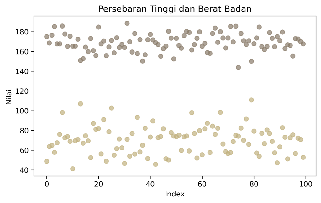
Two-dimensional data exploration is an analytical process aimed at understanding the characteristics and patterns of data with two variables. To extract information from two-dimensional data, the data is typically presented in the form of scatter plots, histograms, and cross-tabulations.
Now imagine, for example, that you have a two-dimensional dataset and you want to identify trends in your data. If you use a histogram, the resulting visualization will be flat and difficult to interpret. The situation is different if you use a scatter plot; the variations in the variables across the data can be more easily understood when using the right visualization.
Multidimensional data exploration
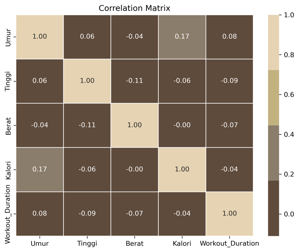
In summary, multidimensional data exploration is an attempt to understand data across various variables. The goal is to identify patterns, structures, relationships, or insights within a dataset that wouldn’t be apparent if viewed through just one or two variables.
Given the many dimensions you want to consider, the best way to examine the relationships between variables is to visualize them using a correlation matrix. Reading it is very simple: for example, if we have row a and column b, the correlation matrix illustrates the relationship between row a and column b. Values in the correlation matrix range from -1 to 1. A value of -1 indicates an opposite relationship, while a value of 1 indicates a strong relationship between the variables, and a value of 0 indicates no relationship.
How to handle data
Using NamedTuples
One handy trick you can use to simplify your data science work is to use the namedtuple package. With this package, you can label the data you’re using, like this:
data = ("Febrian", 25)
print(data[0])  #not sure what this printout is.
If you want to label the data you’re using, you can use a namedtuple, and the result will look like this.
from collections import namedtuple

Person = namedtuple("Person", ["name", "age"])
p = Person("Febrian", 25)

print(p.name)  # It's very clear that what's printed is the name and age
print(p.age)
Data classes
The next point isn’t really that fundamental, but if you use it, the code you write will be neater and more concise. The method in question is data classes—data classes are a way to store data, and the goal is to avoid rewriting the same data over and over again. Let’s jump right into a coding example.
from typing import List

# fungsi cleaning
def clean_text(text: str) -> str:
    text = text.lower()
    text = re.sub(r"http\S+", "", text)
    text = re.sub(r"[^a-zA-Z\s]", "", text)
    return text.strip()

# fungsi sentiment
def simple_sentiment(text: str) -> str:
    positive_words = ["good", "great", "happy", "love", "awesome"]
    negative_words = ["bad", "sad", "hate", "terrible", "angry"]

    score = 0
    for word in positive_words:
        if word in text:
            score += 1
    for word in negative_words:
        if word in text:
            score -= 1

    if score > 0:
        return "positive"
    elif score < 0:
        return "negative"
    else:
        return "neutral"

# CLASS BIASA
class Tweet:
    def __init__(self, id, username, raw_text):
        self.id = id
        self.username = username
        self.raw_text = raw_text

        # manual isi field tambahan
        self.cleaned_text = clean_text(raw_text)
        self.sentiment = simple_sentiment(self.cleaned_text)

    def word_count(self):
        return len(self.cleaned_text.split())

    def is_long_tweet(self):
        return self.word_count() > 10


# =========================
# DATA
# =========================
tweets_data = [
    {"id": 1, "username": "user1", "text": "I love this product! It's awesome 😍"},
    {"id": 2, "username": "user2", "text": "This is bad, I hate it"},
    {"id": 3, "username": "user3", "text": "It's okay, nothing special"},
]

tweets: List[Tweet] = []

for data in tweets_data:
    tweet = Tweet(
        id=data["id"],
        username=data["username"],
        raw_text=data["text"]
    )
    tweets.append(tweet)

# =========================
# OUTPUT
# =========================
for t in tweets:
    print("ID:", t.id)
    print("User:", t.username)
    print("Raw:", t.raw_text)
    print("Cleaned:", t.cleaned_text)
    print("Sentiment:", t.sentiment)
    print("Word Count:", t.word_count())
    print("Long Tweet:", t.is_long_tweet())
    print("-" * 40)
In comparison, here is the code that uses data classes.
from dataclasses import dataclass, field
from typing import List
import re

# fungsi sederhana buat cleaning text
def clean_text(text: str) -> str:
    text = text.lower()
    text = re.sub(r"http\S+", "", text)  # hapus link
    text = re.sub(r"[^a-zA-Z\s]", "", text)  # hapus simbol
    return text.strip()

# fungsi simple sentiment (rule-based)
def simple_sentiment(text: str) -> str:
    positive_words = ["good", "great", "happy", "love", "awesome"]
    negative_words = ["bad", "sad", "hate", "terrible", "angry"]

    score = 0
    for word in positive_words:
        if word in text:
            score += 1
    for word in negative_words:
        if word in text:
            score -= 1

    if score > 0:
        return "positive"
    elif score < 0:
        return "negative"
    else:
        return "neutral"

# DATA CLASS
@dataclass
class Tweet:
    id: int
    username: str
    raw_text: str
    cleaned_text: str = field(init=False)
    sentiment: str = field(init=False)

    def __post_init__(self):
        # otomatis jalan setelah object dibuat
        self.cleaned_text = clean_text(self.raw_text)
        self.sentiment = simple_sentiment(self.cleaned_text)

    def word_count(self) -> int:
        return len(self.cleaned_text.split())

    def is_long_tweet(self) -> bool:
        return self.word_count() > 10


# =========================
# SIMULASI DATA
# =========================
tweets_data = [
    {"id": 1, "username": "user1", "text": "I love this product! It's awesome 😍"},
    {"id": 2, "username": "user2", "text": "This is bad, I hate it"},
    {"id": 3, "username": "user3", "text": "It's okay, nothing special"},
]

# convert ke object data class
tweets: List[Tweet] = []

for data in tweets_data:
    tweet = Tweet(
        id=data["id"],
        username=data["username"],
        raw_text=data["text"]
    )
    tweets.append(tweet)

# =========================
# ANALISIS
# =========================
for t in tweets:
    print("ID:", t.id)
    print("User:", t.username)
    print("Raw:", t.raw_text)
    print("Cleaned:", t.cleaned_text)
    print("Sentiment:", t.sentiment)
    print("Word Count:", t.word_count())
    print("Long Tweet:", t.is_long_tweet())
    print("-" * 40)

# =========================
# SUMMARY
# =========================
positive = sum(1 for t in tweets if t.sentiment == "positive")
negative = sum(1 for t in tweets if t.sentiment == "negative")
neutral = sum(1 for t in tweets if t.sentiment == "neutral")

print("Summary:")
print("Positive:", positive)
print("Negative:", negative)
print("Neutral:", neutral)
What’s the difference? Without data classes, you have to write the _init_ method manually and define all attributes one by one. With data classes, you can write cleaner code. Data classes allow you to automatically generate the (_init_, _repr_, and _eq_) methods. All that’s left is to focus on building the logic.
Data cleaning
The data you’ll be working with is generally raw and highly unstructured, so you’ll need to set aside plenty of time to clean it until it’s truly ready for use. The first step in data cleaning is to identify the purpose of your data analysis. Once you’ve identified your objective, determine the data you need, and then proceed with the data cleaning process. Essentially, the data cleaning process involves checking for missing values, outliers, and bad data in the dataset that we will use.
When you discover that there are missing values in your data, there are several things you can do. The first is to delete them, and the next is to fill them in with the mean, median, or you can generate data based on previous trends.
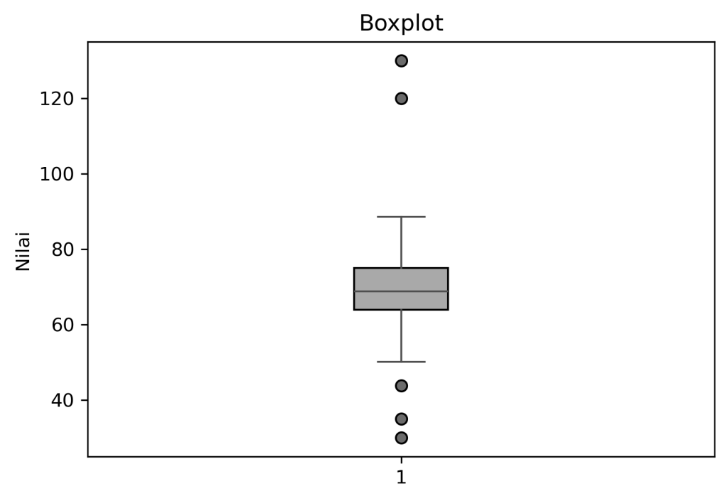
The next issue that comes up is outliers; simply put, an outlier is a data point that deviates from the pattern. Outliers can be ignored if there are only a small number of them, as they are considered to have no impact on the analysis process. However, if there are many outliers, you’ll need to take additional steps to address them—for example, by using a robust model that handles outliers and applying data transformations. To detect outliers, you can use boxplot visualizations.
The last point is how to handle bad data. By “bad data,” I mean data that you have already cleaned of missing values and outliers but still contains information that is not needed for analysis. What you can do is standardize the data formatting to ensure consistency in the resulting data. You can also perform filtering by removing unnecessary data.
Manipulating data
Data manipulation is the process of processing or transforming data to align with research objectives in order to produce optimal analysis. Data that has been cleaned through the data cleansing process can then proceed to the next stage.
There are several methods for manipulating data; the following are some of them: filtering data, grouping, joining tables, and creating new columns. However, keep in mind that not all of these methods need to be used when manipulating data; tailor your approach to the objectives of your research.
- Filtering = A method for selecting data based on specific needs (for example, out of 1,000 records, you only need data for customers over the age of 25).
- Grouping = A method for grouping data and then calculating its statistics.
- Table join = If there is duplicate data located in different rows, you can use a table join to combine them.
- Create a new column = You create a new column based on your needs (for example, you need data on customer age after adding 5 years)
Rescaling
When building a machine learning model, we sometimes encounter models that are sensitive to variations in the input data. We need to apply a rescaling method to produce an optimal model. Rescaling is a process of adjusting the scale of values in a dataset to a specific range without altering its underlying patterns or distribution.
For example, suppose you have data on weight and height at a company, with two different units: centimeters and inches. If we have features with different scales, some machine learning algorithms may be biased toward features with larger values. Therefore, rescaling is necessary.
| Name | Weight (kg) | Height (cm) | Height (inches) |
|---|---|---|---|
| A | 50 | 160 | 63 |
| B | 70 | 170 | 67 |
| C | 90 | 180 | 71 |
Rescaling is typically performed using the min-max method. Here is the formula for the min-max method. After applying this formula, the table will look like this:
| Name | Weight (scaled) | Height cm (scaled) | Height inci (scaled) |
|---|---|---|---|
| A | 0.00 | 0.00 | 0.00 |
| B | 0.50 | 0.50 | 0.50 |
| C | 1.00 | 1.00 | 1.00 |
After rescaling, the model will treat the data more fairly. Some models are sensitive to large gaps in data values, including KNN, SVM, and clustering. You can use rescaling if your data contains features with vastly different scales.
Dimensionality reduction
Sometimes the data is just too overwhelming. Have you ever tried visualizing it? Then you realize that you can already make out the patterns with just 70% of the data. For problems like this, you can use dimensionality reduction. By definition, dimensionality reduction is a method for reducing the number of features or variables in a dataset while retaining the essential information. In other words, it’s like cutting out the unnecessary data and keeping only the important parts.
The purpose of dimensionality reduction is to eliminate unnecessary data noise, so that the resulting model runs faster and reduces overfitting (a model that is too “smart”—meaning it performs well only on the training dataset but is prone to errors when tested on other datasets).


That concludes my explanation of how to approach data science work, from the data preparation process to the final presentation. I hope this provides some useful information for readers. If you’d like to read my other posts, please visit the blog section.
Warm regrads
Febrian
Also read: The catalyst